I.3.8.2: Convergence to Incorrect Solutions
Convergence needs not be towards a minimum, even if the function is convex. This example is an elaboration of the one in Abatzoglou and O'Donnell [1982].
Let To compute we do the usual Chebyshev calculations. If and we must have , for some and . Moreover . Thus The solution is , , , and . Thus the best linear Chebyshev approximation to on the unit interval is which has function value ,
Now use coordinate decent. Start with Then and Thus , and we have convergence after a single cycle to a point for which .
This example can be analyzed in more in detail. First we compute the best constant (zero degree polynomial) approximation to . The function is a convex quadratic with roots at zero and , with a mimimum equal to at .
We start with the simple rule that the best constant approximation is the average of the maximum and the minimum on the interval. We will redo the calculations later on, using a different and more general approach.
Case A: If then is non-negative and increasing in the unit interval, and thus .
Case B: If then attains its minimum at in the unit interval, and its maximum at one, thus .
Case C: If then still attains its minimum at in the unit interval, but now the maximum is at zero, and thus .
Case D: If then is non-positive and decreasing in the unit interval, and thus again .
We can derive the same results, and more, by using a more general approach. First Since is convex, we see Now has a minimum at equal to . This is the minimum over the closed interval if , otherwise the minimum occurs at one of the boundaries. Thus and It follows that It is more complicated to compute , because the corresponding Chebyshev approximation problem does not satisfy the Haar condition, and the solution may not be unique.
We make the necessary calculations, starting from the left. Define . For we have . Define and . Then Note that for all . If then has a minimum equal to for all in . Now if and only if . Thus for we have
Switch to . For we have . We have if and only if . The discriminant of this quadratic is , which means that if we have everywhere. If define and as the two roots of the quadratic. Now Clearly . If then also and thus on . If then has a minimum at . Thus if we have
Next , which is equal to for . If then everywhere. If define and as . Then If then we have a minimum of at . Thus if we find
And finally we get back to again at the right hand side of the real line. We have a minimum if , i.e. . In that case
So, in summary,
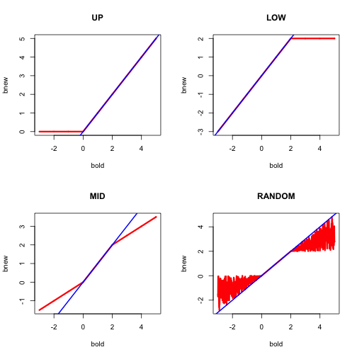
We now have enough information to write a simple coordinate descent algorithm. Of course such an algorithm would have to include a rule to select from the set of minimizers if the minimers are not unique. In our R implementation in ccd.R we allow for different rules. If the minimizers are an interval, we always choose the smallest point, or always to largest point, or always the midpoint, or a uniform draw from the interval. We shall see in our example that these
different options have a large influence on the approximation the algorithm converges too, in fact even on what the algorithm considers to be desirable points.
We give the function that transforms into with the four different selection rules in Figure 1.
The function is in red, the line in blue. Thus over most of the region of interest the algorithm does not change the slope, which means it converges in a single iteration to an incorrect solution. It needs more iterations only for the midpoint and random selection rules if started outside
