I.4.3.4: Rayleigh Quotient

The problem is to minimize the Rayleigh quotient $$\lambda(x)=\frac{x'Ax}{x'Bx}$$ over all $x.$ Here $A$ and $B$ are known matrices, with $B$ positive definite.

If we update $x$ to $\tilde x=x+\theta e_i,$ with $e_i$ a unit vector, then $$\lambda(\tilde x)= \frac{\theta^2a_{ii}+2\theta x'a_i+x'Ax} {\theta^2b_{ii}+2\theta x'b_i+x'Bx}.$$ Think of this as a continous rational function $\gamma$ of the single variable $\theta$, which we have to minimize. Clearly $\gamma$ has a horizontal asymptote, with $$\lim_{\theta\rightarrow+\infty}\gamma(\theta)= \lim_{\theta\rightarrow-\infty}\gamma(\theta)=\frac{a_{ii}}{b_{ii}}.$$ Also $$\mathcal{D}\gamma(\theta)=\frac{2Q(\theta)}{P^2(\theta)},$$ with $$P(\theta)\mathop{=}\limits^{\Delta}\theta^2b_{ii}+2\theta x'b_i+x'Bx,$$ and $$Q(\theta)\mathop{=}\limits^{\Delta}\theta^2(a_{ii}x'b_i-b_{ii}x'a_i) +\theta(a_{ii}x'Bx-b_{ii}x'Ax)+ (x'a_ix'Bx-x'b_ix'Ax).$$ In addition $$\mathcal{D}^2\gamma(\hat\theta)=2\frac{P^2(\theta)\mathcal{D}Q(\theta)-Q(\theta)\mathcal{D}P^2(\theta)}{P^4(\theta)},$$ and thus $\mathbf{sign}(\mathcal{D}\gamma(\theta))= \mathbf{sign}(Q(\theta))$ and at values where $Q(\theta)=0$ we have $\mathbf{sign}(\mathcal{D}^2\gamma(\theta))= \mathbf{sign}(\mathcal{D}Q(\theta))$.

We now distinguish three cases.

1. First, $\gamma$ can be a constant function, everywhere equal to $\frac{a_{ii}}{b_{ii}}$. This happens only if $x=0$ or $x=e_i$, which makes $Q(\theta)=0$ for all $\theta$. In this case we do not update, and just go to the next $i$.
2. Second, $Q$ can have a zero quadratic term. If we make sure that $\frac{x'Ax}{x'Bx}<\frac{a_{ii}}{b_{ii}}$ then the unique solution of the linear equation $Q(\theta)=0$ satisfies $\mathcal{D}^2\gamma(\theta)>0$, and consequently corresponds with the unique minimum of $\gamma$. Updating $x$ guarantees that we will have $\frac{x'Ax}{x'Bx}<\frac{a_{ii}}{b_{ii}}$ for all subsequent iterations. If we happen to start with or wind up in a point with a zero quadratic term and with $\frac{x'Ax}{x'Bx}>\frac{a_{ii}}{b_{ii}}$ then $\gamma$ does not have a minimum and coordinate descent fails.
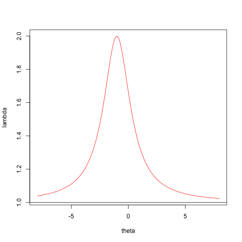
3. If $Q$ is a proper quadratic then $\gamma$ is either increasing at both infinities or decreasing at both infinities. In the first case, when $Q$ is a convex quadratic, $\gamma$ increases from the horizontal asymptote to the maximum, then decreases to the minimum, and then increases again to the horizontal asymptote. In the second case, with $Q$ a concave quadratic, $\gamma$ decreases from the horizontal asymptote to the minimum, then increases to the maximum, and then decreases again to the horizontal asymptote. In either case it has two extremes, one minimum and one maximum, corresponding to the roots of the quadratic $Q$. This also shows that if $Q$ is a proper quadratic, then it always has two distinct real roots.

Here is some simple code to illustrate the cases distinguished above. We have a simple function to compute $\lambda$.

a <-  matrix (-1, 3, 3)
diag (a) <- 1
b <-  diag (3)
x <- c(1, 1, -1)
zseq <- seq (-8, 8, length = 100)
png("myOne.png")
plot (zseq, fRayleigh (zseq, 1, x, a, b),type="l",cex=3,col="RED",xlab="theta",ylab="lambda")
abline(h=a[1,1] / b[1,1])
dev.off()
x <- c(1,0,1)
png("myTwo.png")
plot (zseq, fRayleigh (zseq, 2, x, a, b),type="l",cex=3,col="RED",xlab="theta",ylab="lambda")
abline(h=a[2,2] / b[2,2])
dev.off()

For Case 2 we see that $\gamma$ has no minimum, and CCD fails. For Case 3, which is of course the usual case, there are no problems.

$$\fbox{Insert Figure 1 here}$$ $$\fbox{Insert Figure 2 here}$$

The coordinate descent method can obviously take sparseness into account, and it can easily be generalized to separable constraints on the elements of $x,$ such as non-negativity. Note that it also can be used to maximize the Rayleigh quotient, simply by taking the other root of the quadratic. Or, alternatively, we can interchange $A$ and $B$.

The second derivative of the Rayleigh quotient at a stationary point normalized by $x'Bx=1$ is simply $$\mathcal{D}^2\lambda(x)=2(A-\lambda(x)B).$$ This is singular and thus the product form of the derative of the algorithmic map has largest eigenvalue equal to one, corresponding with the eigenvector $x$. Singularity of the Hessian is due, of course, to the fact that $\lambda$ is homogenous of degree zero, and rescaling $x$ does not change the value of the objective function. We can use this to our advantage. Suppose we normalize $x$ to $x'Bx=1$, after each coordinate descent cycle. This will not change the function values computed by the algorithm, but is changes the algorithmic map. The derivative of the modified map is $$\overline{\mathcal{M}}(x)=(I-yy'B)\mathcal{M}(x),$$ which has the same eigenvalues and eigenvectors as $\mathcal{M}(x)$, except for $\overline{\mathcal{M}}(x)x=0$, while $\mathcal{M}(x)x=1$.

Figure 1: Case 2 -- CCA Fails </center>

Figure 2: Case 2 -- CCA Works </center>