Univariate Cubics

Suppose the problem is to minimize the cubic $f(x)=\alpha+\beta x+\frac12\gamma x^2+\frac16\delta x^3$ with $\delta\not= 0$ . Since the cubic has no majorizers, we will find a local majorizer on the interval $[A,B]$ .

From $f''(x)=\gamma+\delta x$ we see that $K(A,B)\mathop{=}\limits^{\Delta}\max_{A\leq z\leq B} f''(z)=\gamma+\begin{cases}\delta B&\text{ if }\delta>0,\\ \delta A&\text{ if }\delta<0.\end{cases}$ and thus, if $y\in[A,B]$ , $f(x)\leq f(y)+f'(y)(x-y)+\frac12 K(A,B)(x-y)^2$ over $A\leq x\leq B$ .

If $K(A,B)>0$ the majorizing quadratic has a minimum at $x=y-\frac{\beta+\gamma y+\frac12\delta y^2}{K(A,B)}$ This minimum can, of course, be outside the interval $[A,B]$ , in which case the minimum of the quadratic is attained at one of the end-points. The minimum of the quadratic can be in the interval, but the function value at the minimum of the quadratic can be larger than the function value at one of the end-points. In that case, again, the majorization algorithm chooses one of the end-points. If $K(A,B)\leq 0$ the majorizer does not have a minimum and thus the minimum on the interval is attained at either $A$ or $B$ . Code in R is in the file cubicBound.R.

[Insert cubicBound.R Here](../code/cubicBound.R)

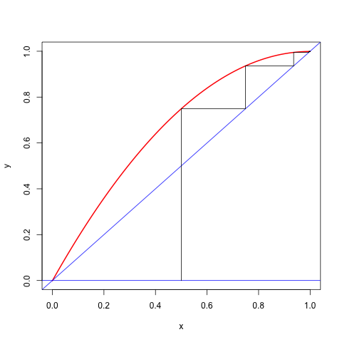
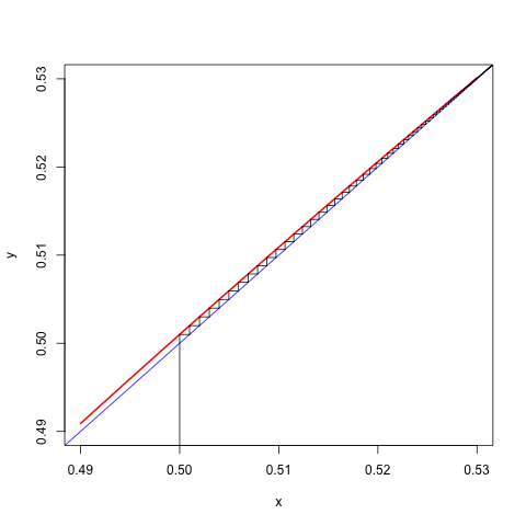
If the iterations stay in the interior of the interval they converge to a local minimum at $\hat x$ with rate $\kappa=1-\frac{\gamma+\delta\hat x}{K(A,B)}$

Consider, for example, the cubic $f(x)=\frac13 x^3-\frac12 x^2+cx$ , where $0\leq c\leq\frac14$ . The function has a local maximum at $\frac12-\frac12\sqrt{1-4c}$ and a local minimum at $\frac12+\frac12\sqrt{1-4c}$ . Both are in the unit interval. The majorization algorithm, using $K(0,1)=1$ , has the update rule $x^{(k+1)}=-(x^{(k)})^2+2x^{(k)}-c.$ If started in the interval $(\frac12-\frac12\sqrt{1-4c},\frac12+\frac12\sqrt{1-4c})$ the algorithm converges monotonically to the local minimum at $\frac12+\frac12\sqrt{1-4c}$ with rate $\kappa=1-\sqrt{1-4c}$ , which is close to zero if $c$ is close to zero and close to one if $c$ is close to $\frac14$ . Here are two runs, the first one is fast, with $c=.001$ , the second one is slow, with $c=.249$ .

> cubicBound(c(0,.001,-.5,1/3),0,1)
Iteration:    1 fold:   -0.08283333 fnew:   -0.13968825 xold:    0.50000000 xnew:    0.74900000
Iteration:    2 fold:   -0.13968825 fnew:   -0.16376999 xold:    0.74900000 xnew:    0.93599900
Iteration:    3 fold:   -0.16376999 fnew:   -0.16565882 xold:    0.93599900 xnew:    0.99490387
Iteration:    4 fold:   -0.16565882 fnew:   -0.16566717 xold:    0.99490387 xnew:    0.99897403
Iteration:    5 fold:   -0.16566717 fnew:   -0.16566717 xold:    0.99897403 xnew:    0.99899895
Iteration:    6 fold:   -0.16566717 fnew:   -0.16566717 xold:    0.99899895 xnew:    0.99899900
$itel
[1] 6

$f
[1] -0.1656672

$x
[1] 0.998999

> cubicBound(c(0,.249,-.5,1/3),0,1)
Iteration:    1 fold:    0.04116667 fnew:    0.04116567 xold:    0.50000000 xnew:    0.50100000
Iteration:    2 fold:    0.04116567 fnew:    0.04116467 xold:    0.50100000 xnew:    0.50199900
Iteration:    3 fold:    0.04116467 fnew:    0.04116368 xold:    0.50199900 xnew:    0.50299500
Iteration:    4 fold:    0.04116368 fnew:    0.04116270 xold:    0.50299500 xnew:    0.50398603
Iteration:    5 fold:    0.04116270 fnew:    0.04116174 xold:    0.50398603 xnew:    0.50497015
...
...
Iteration:   89 fold:    0.04114559 fnew:    0.04114559 xold:    0.53141255 xnew:    0.53142580
Iteration:   90 fold:    0.04114559 fnew:    0.04114559 xold:    0.53142580 xnew:    0.53143822
Iteration:   91 fold:    0.04114559 fnew:    0.04114559 xold:    0.53143822 xnew:    0.53144986
Iteration:   92 fold:    0.04114559 fnew:    0.04114559 xold:    0.53144986 xnew:    0.53146077
Iteration:   93 fold:    0.04114559 fnew:    0.04114559 xold:    0.53146077 xnew:    0.53147099
Iteration:   94 fold:    0.04114559 fnew:    0.04114559 xold:    0.53147099 xnew:    0.53148056
$itel
[1] 94

$f
[1] 0.04114559

$x
[1] 0.5314806

We can also make cobweb plots for these two runs. They are in the figures below. $\fbox{Insert Figure 1 here}$ $\fbox{Insert Figure 2 here}$

Figure 1: Cobweb Plot for c=0.001 </center>

Figure 2: Cobweb Plot for c=0.249</center>