II.1.2.3: Majorization Algorithm
The basic idea of a majorization algorithm is simple: it is the augmentation algorithm applied to the majorization function.
Suppose our current best approximation to the minimum of is , and we have a that majorizes on in . If already minimizes we stop, otherwise we update to by minimizing over .
If we do not stop, we have the sandwich inequality and in the case of strict majorization even
We then select a new function that majorizes on at . Repeating these steps produces a decreasing sequence of function values, and the usual compactness and continuity conditions guarantee convergence of both sequences and .
Here is an artificial example, chosen because of its simplicity. Consider Because we see that is a suitable majorization function. The majorization algorithm is
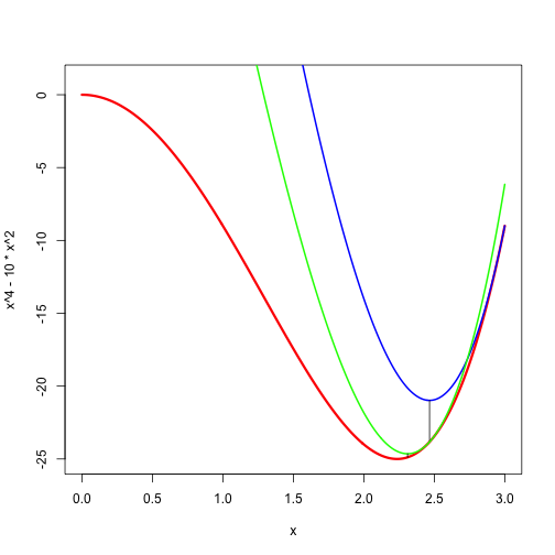
The first iterations of the algorithm are illustrated in Figure 1. We start with where is . Then is the blue function. It is minimized at where and We then majorize by using the green function , which has its minimum at about equal to about The corresponding value of at this point is about Thus we are rapidly getting close to the local minimum at with value The linear convergence rate at the stationary point is

Table 1 show the iterations to convergence, with an estimate of the iteration radius in the last column.
## Iteration:    1 fold:   -9.00000000 fnew:  -23.82883884 xold:    3.00000000 xnew:    2.46621207 ratio:    0.00000000
## Iteration:    2 fold:  -23.82883884 fnew:  -24.88612919 xold:    2.46621207 xnew:    2.31029165 ratio:    0.32250955
## Iteration:    3 fold:  -24.88612919 fnew:  -24.98789057 xold:    2.31029165 xnew:    2.26054039 ratio:    0.32971167
## Iteration:    4 fold:  -24.98789057 fnew:  -24.99867394 xold:    2.26054039 xnew:    2.24419587 ratio:    0.33212463
## Iteration:    5 fold:  -24.99867394 fnew:  -24.99985337 xold:    2.24419587 xnew:    2.23877400 ratio:    0.33293027
## Iteration:    6 fold:  -24.99985337 fnew:  -24.99998373 xold:    2.23877400 xnew:    2.23696962 ratio:    0.33319896
## Iteration:    7 fold:  -24.99998373 fnew:  -24.99999819 xold:    2.23696962 xnew:    2.23636848 ratio:    0.33328854
## Iteration:    8 fold:  -24.99999819 fnew:  -24.99999980 xold:    2.23636848 xnew:    2.23616814 ratio:    0.33331840
## Iteration:    9 fold:  -24.99999980 fnew:  -24.99999998 xold:    2.23616814 xnew:    2.23610137 ratio:    0.33332836
## Iteration:   10 fold:  -24.99999998 fnew:  -25.00000000 xold:    2.23610137 xnew:    2.23607911 ratio:    0.33333167
## Iteration:   11 fold:  -25.00000000 fnew:  -25.00000000 xold:    2.23607911 xnew:    2.23607169 ratio:    0.33333278
## Iteration:   12 fold:  -25.00000000 fnew:  -25.00000000 xold:    2.23607169 xnew:    2.23606921 ratio:    0.33333315
## Iteration:   13 fold:  -25.00000000 fnew:  -25.00000000 xold:    2.23606921 xnew:    2.23606839 ratio:    0.33333327
## Iteration:   14 fold:  -25.00000000 fnew:  -25.00000000 xold:    2.23606839 xnew:    2.23606811 ratio:    0.33333331
## Iteration:   15 fold:  -25.00000000 fnew:  -25.00000000 xold:    2.23606811 xnew:    2.23606802 ratio:    0.33333333
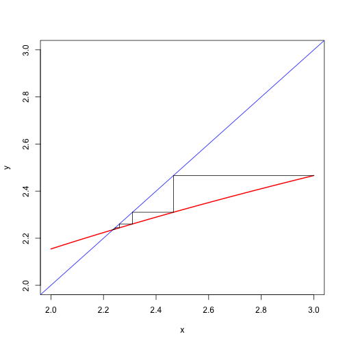
We also show the cobwebplot (see section 14.11.2) for the iterations, which illustrates the decrease of the difference between subsequent iterates.
